Step 8. Along-tract profiles

Each cleaned bundle is converted to a 100-point profile of a scalar map: fractional anisotropy (FA) from the tensor fit; the neurite density index (NDI), orientation dispersion index (ODI) and free-water fraction (FWF) from neurite orientation dispersion and density imaging (NODDI; Zhang et al., 2012); or any other map on the diffusion grid. Profiling follows the tract-profile approach of Yeatman et al. (2012) as implemented in DIPY (Garyfallidis et al., 2014).

Two operations make profiles comparable across participants. First, because streamlines in a tractogram file may run in either direction, each bundle is oriented against its QuickBundles centroid (Garyfallidis et al., 2012; threshold=np.inf, yielding one cluster), and the centroid is itself oriented so that it begins at the end nearer the warped seed region. Node 0 therefore corresponds to the seed end and node 99 to the target end in every participant. Second, afq_profile with gaussian_weights weights each streamline's contribution at a node by its Mahalanobis distance from the bundle core, reducing the influence of outlying streamlines.

Procedure

metric = AveragePointwiseEuclideanMetric(ResampleFeature(nb_points=100))
centroid = QuickBundles(threshold=np.inf, metric=metric).cluster(streamlines).centroids[0]
if distance(centroid[0], seed_centre) > distance(centroid[-1], seed_centre):
    centroid = centroid[::-1]                       # node 0 at the seed end
oriented = orient_by_streamline(streamlines, centroid)
weights = gaussian_weights(oriented, n_points=100)
profile = afq_profile(data, oriented, affine, n_points=100, weights=weights)

The METRICS dictionary in the script specifies the scalar maps; the script writes one long-format CSV per tract with one column per metric. Processing takes roughly 10 s per participant and tract.

Script 08_node_profiles.py (120 lines)

08_node_profiles.py

#!/usr/bin/env python3
"""Step 8. Sample each scalar map at 100 nodes along the cleaned bundle (AFQ tract profile).

Inputs, per participant:
    $OUT/<s>/tckgen/<TRACT>/<TRACT>_<CUTOFF>_cleaned.tck   cleaned bundle (Step 6)
    $OUT/<s>/rois/<TRACT>_seed_diff.nii.gz                 seed region (Step 2); node 0 end
    $PROJECT/dwi/<s>/fa.nii.gz                             FA map
    $PROJECT/noddi/<s>/fit_*.nii.gz                        NODDI maps (Step 8a, optional)
Output: $OUT/nodewise/<TRACT>_nodewise_all_subjects.csv (long format; Step 8b pivots it)
Run:    source 00_config.sh && python 08_node_profiles.py
"""
import os
import sys
from pathlib import Path

import nibabel as nib
import numpy as np
import pandas as pd
from dipy.io.image import load_nifti
from dipy.io.streamline import load_tractogram
from dipy.segment.clustering import QuickBundles
from dipy.segment.featurespeed import ResampleFeature
from dipy.segment.metricspeed import AveragePointwiseEuclideanMetric
from dipy.stats.analysis import afq_profile, gaussian_weights
from dipy.tracking.streamline import Streamlines, orient_by_streamline


# Read one variable exported by 00_config.sh, or stop with a hint.
def env(name):
    if name not in os.environ:
        sys.exit(f"{name} is not set: run `source 00_config.sh` first")
    return os.environ[name]


# TRACT and CUTOFF go into file names, so they must match what Steps 5 and 6 ran with.
PROJECT = Path(env("PROJECT"))
OUT = Path(env("OUT"))
TRACT = env("TRACT")
CUTOFF = env("CUTOFF")
# bash cannot export an array, so the ID list is re-read from the file.
SUBJECTS = Path(env("SUBJECTS_FILE")).read_text().split()

# 100 nodes is the AFQ convention; Step 9a's quartiles and Step 9c's blocks of 100 assume it.
N_NODES = 100
# A real bundle has hundreds of streamlines; a handful means tracking or cleaning failed.
MIN_STREAMLINES = 5
METRICS = {
    "FA": "dwi/{s}/fa.nii.gz",
    "NDI": "noddi/{s}/fit_NDI_modulated.nii.gz",
    "ODI": "noddi/{s}/fit_ODI_modulated.nii.gz",
    "FWF": "noddi/{s}/fit_FWF.nii.gz",
}


unavailable = [m for m, template in METRICS.items()
               if not any((PROJECT / template.format(s=s)).exists() for s in SUBJECTS)]
for m in unavailable:
    print(f"metric {m}: no image found for any participant; not profiled")
    del METRICS[m]
if not METRICS:
    sys.exit("no scalar images found")


def seed_centre_mm(s):
    """Centre of mass of the warped seed region, in scanner (mm) coordinates."""
    img = nib.load(str(OUT / s / "rois" / f"{TRACT}_seed_diff.nii.gz"))
    voxels = np.argwhere(img.get_fdata() > 0)
    return nib.affines.apply_affine(img.affine, voxels.mean(axis=0))


def orient_seed_to_target(streamlines, seed_mm):
    """Orient all streamlines alike, with node 0 at the seed end."""
    # threshold=np.inf: one cluster, so centroids[0] is the mean streamline of the whole bundle.
    metric = AveragePointwiseEuclideanMetric(ResampleFeature(nb_points=N_NODES))
    centroid = QuickBundles(threshold=np.inf, metric=metric).cluster(streamlines).centroids[0]
    # The centroid may run either way; flip it so node 0 is the seed end in every participant.
    starts_at_target = (np.linalg.norm(centroid[0] - seed_mm)
                        > np.linalg.norm(centroid[-1] - seed_mm))
    if starts_at_target:
        centroid = centroid[::-1]
    return Streamlines(orient_by_streamline(streamlines, centroid))


# Sample one scalar map along the oriented bundle; one value per node.
def profile(image, streamlines, weights):
    data, affine = load_nifti(str(image))
    return afq_profile(data, streamlines, affine, n_points=N_NODES, weights=weights)


# --- Main loop, one participant at a time ---
rows = []
for s in SUBJECTS:
    tck = OUT / s / "tckgen" / TRACT / f"{TRACT}_{CUTOFF}_cleaned.tck"
    maps = {m: PROJECT / template.format(s=s) for m, template in METRICS.items()}
    missing = [str(p) for p in [tck, *maps.values()] if not p.exists()]
    if missing:
        print(f"[{s}] SKIP: missing {missing[0]}")
        continue

    # Any map can be the grid; bbox_valid_check=False accepts points outside it, as in Step 6.
    reference = next(iter(maps.values()))
    streamlines = load_tractogram(str(tck), str(reference), bbox_valid_check=False).streamlines
    if len(streamlines) < MIN_STREAMLINES:
        print(f"[{s}] SKIP: {len(streamlines)} streamlines")
        continue

    # Orient first; the weights are per node, so node i must line up across streamlines.
    # Weights depend on geometry only, so one matrix serves every metric.
    streamlines = orient_seed_to_target(streamlines, seed_centre_mm(s))
    weights = gaussian_weights(streamlines, n_points=N_NODES)
    profiles = {m: profile(p, streamlines, weights) for m, p in maps.items()}
    for node in range(N_NODES):
        rows.append({"Subject": s, "Tract": TRACT, "Node": node,
                     **{m: float(profiles[m][node]) for m in METRICS}})
    print(f"[{s}] {len(streamlines)} streamlines, {N_NODES} nodes, {len(METRICS)} metrics")

out = OUT / "nodewise" / f"{TRACT}_nodewise_all_subjects.csv"
out.parent.mkdir(parents=True, exist_ok=True)
pd.DataFrame(rows).to_csv(out, index=False)
print(f"DONE -> {out}  ({len(rows) // N_NODES} participants)")

Node range

Nodes near the ends of the profile (0 to 4 and 95 to 99) lie in or adjacent to gray matter and are affected by partial-volume contamination from the seed and target regions. Deep white matter spans approximately nodes 25 to 75. Whether end nodes are trimmed should be decided before modelling.

NODDI inputs

NODDI is fitted with AMICO (Daducci et al., 2015) on the eddy-corrected data; the script 08a_noddi_fit.py, shown below, performs the fit. The modulated NDI and ODI maps (fit_NDI_modulated.nii.gz, fit_ODI_modulated.nii.gz), which incorporate the tissue-weighted partial-volume correction of Parker et al. (2021), are used for profiling; FWF has no modulated form and fit_FWF.nii.gz is used. Settings used in the example dataset were bStep=200 during scheme conversion (rounding jittered b-values), b0_thr=100, doSaveModulatedMaps=True, doComputeRMSE=True and BLAS_nthreads=1. By default AMICO writes its response kernels to a directory shared by all participants, and concurrent jobs then delete one another's files; the script instead generates the kernels in a working directory for each participant, so several instances can be run at once on different participants (python 08a_noddi_fit.py sub-01 sub-02). AMICO also empties its output directory when saving, so nothing else should be stored there.

When NODDI is sampled within a gray-matter region (for example the hippocampus), the model should be refitted with the gray-matter intrinsic parallel diffusivity (approximately 1.1 × 10⁻³ mm²/s rather than the white-matter default of 1.7 × 10⁻³ mm²/s) by setting NODDI_DPAR=1.1e-3; the script then writes to $PROJECT/noddi_gm so that the white-matter maps are retained. The white-matter fit is not appropriate in gray matter and the two fits can yield different results.

Script 08a_noddi_fit.py (88 lines)

08a_noddi_fit.py

#!/usr/bin/env python3
"""Step 8a. Fit NODDI with AMICO so Step 8 can profile NDI, ODI and FWF along the bundle.

Inputs:  $PROJECT/dwi/<subj>/{data.nii.gz, bvals, bvecs, nodif_brain_mask.nii.gz}
Outputs: $PROJECT/noddi/<subj>/fit_{NDI,ODI,FWF,NDI_modulated,ODI_modulated,RMSE}.nii.gz
         (noddi_gm/ instead when NODDI_DPAR is set); work/<subj>/ is scratch, safe to delete
Run:     source 00_config.sh && python 08a_noddi_fit.py [sub-01 sub-02 ...]
"""
import os
import sys
from pathlib import Path

N_THREADS = os.environ.get("NODDI_NTHREADS", "4")
# numpy's BLAS reads these at import time, and importing amico imports numpy.
os.environ["OPENBLAS_NUM_THREADS"] = N_THREADS     # must be set before amico is imported
os.environ["OMP_NUM_THREADS"] = N_THREADS

import amico


# Read a variable exported by 00_config.sh, or stop with a message naming it.
def env(name):
    if name not in os.environ:
        sys.exit(f"{name} is not set: run `source 00_config.sh` first")
    return os.environ[name]


PROJECT = Path(env("PROJECT"))
FORCE = os.environ.get("FORCE", "0") == "1"
SUBJECTS = sys.argv[1:] or Path(env("SUBJECTS_FILE")).read_text().split()

# dPar is fixed, not fitted, so it must suit the tissue: 1.7e-3 white matter, 1.1e-3 gray.
D_PAR = os.environ.get("NODDI_DPAR")     # mm2/s; unset = AMICO default for white matter
D_ISO = 3.0e-3                           # isotropic (free water) diffusivity, mm2/s
B0_THRESHOLD = 100                       # volumes with b below this are treated as b = 0
B_STEP = 200                             # b-values are rounded to the nearest multiple

STUDY = PROJECT / ("noddi_gm" if D_PAR else "noddi")
STUDY.mkdir(parents=True, exist_ok=True)
# One-off: caches AMICO's rotation matrices in ~/.dipy, so only the first call is slow.
amico.setup()

for s in SUBJECTS:
    dwi_dir = PROJECT / "dwi" / s
    dwi = dwi_dir / "data.nii.gz"
    bvals = dwi_dir / "bvals"
    bvecs = dwi_dir / "bvecs"
    mask = dwi_dir / "nodif_brain_mask.nii.gz"
    out = STUDY / s

    if (out / "fit_NDI_modulated.nii.gz").exists() and not FORCE:
        print(f"[{s}] NODDI maps exist")
        continue
    missing = [p.name for p in (dwi, bvals, bvecs, mask) if not p.exists()]
    if missing:
        print(f"[{s}] SKIP: missing {', '.join(missing)}")
        continue
    # AMICO clears the output directory on save, so the scheme and kernels live in work/.
    # One work directory per participant: with AMICO's shared default, concurrent runs collide.
    work = STUDY / "work" / s
    work.mkdir(parents=True, exist_ok=True)
    out.mkdir(parents=True, exist_ok=True)

    scheme = work / f"{s}.scheme"
    amico.util.fsl2scheme(str(bvals), str(bvecs), str(scheme), bStep=B_STEP)

    # Evaluation(study_dir, participant, output_path): the maps go straight to noddi/<subj>/.
    ae = amico.Evaluation(str(STUDY), s, str(out))
    # BLAS_nthreads=1 so the two thread counts do not multiply and oversubscribe the machine.
    ae.set_config("nthreads", int(N_THREADS))
    ae.set_config("BLAS_nthreads", 1)
    ae.set_config("doSaveModulatedMaps", True)
    ae.set_config("doComputeRMSE", True)
    ae.load_data(str(dwi), str(scheme), str(mask), b0_thr=B0_THRESHOLD)

    ae.set_model("NODDI")
    ae.set_config("ATOMS_path", str(work / "kernels"))     # after set_model, which resets it
    # model.set(dPar, dIso, IC_VFs, IC_ODs, isExvivo); only dPar changes here.
    if D_PAR:
        ae.model.set(float(D_PAR), D_ISO, ae.model.IC_VFs, ae.model.IC_ODs, False)
    # regenerate=True so a half-written kernel set from a killed run is never picked up.
    ae.generate_kernels(regenerate=True)
    ae.load_kernels()
    ae.fit()
    ae.save_results()
    print(f"[{s}] NODDI maps written (dPar = {ae.model.dPar})")

print(f"DONE -> {STUDY}")

Analysis file

Inference in Step 9 reads a wide file with one row per participant: the covariates and outcomes, the streamline count and mean length of the cleaned bundle from Step 6, and the 100 node values as columns <METRIC>_0 to <METRIC>_99. The script 08b_build_analysis_csv.py, shown below, builds one such file per tract and metric from the long profile CSV, the tract statistics file and a participant-level covariates file (COVARIATES_CSV in the configuration; columns Subject plus covariates and outcomes).

Script 08b_build_analysis_csv.py (48 lines)

08b_build_analysis_csv.py

#!/usr/bin/env python3
"""Step 8b. Reshape the Step 8 node profiles to one row per participant and join covariates.
Inputs:  $OUT/nodewise/<TRACT>_{nodewise_all_subjects,tract_stats}.csv (Steps 8 and 6)
         $COVARIATES_CSV (Subject, covariates, outcomes)
Output:  $OUT/analysis/<TRACT>__<METRIC>__analysis.csv, one per metric, named as Step 9 expects
Run:     source 00_config.sh && python 08b_build_analysis_csv.py
"""
import os
import sys
from pathlib import Path

import pandas as pd


# Read one exported config variable or stop; exports need `source 00_config.sh`, not `bash`.
def env(name):
    if name not in os.environ:
        sys.exit(f"{name} is not set: run `source 00_config.sh` first")
    return os.environ[name]


OUT = Path(env("OUT"))
TRACT = env("TRACT")

# Subject as str in all three files: all-digit IDs keep leading zeros and the merges match.
profiles = pd.read_csv(OUT / "nodewise" / f"{TRACT}_nodewise_all_subjects.csv",
                       dtype={"Subject": str})
tract_stats = pd.read_csv(OUT / "nodewise" / f"{TRACT}_tract_stats.csv", dtype={"Subject": str})
covariates = pd.read_csv(env("COVARIATES_CSV"), dtype={"Subject": str})
metrics = [c for c in profiles.columns if c not in ("Subject", "Tract", "Node")]

analysis_dir = OUT / "analysis"
analysis_dir.mkdir(parents=True, exist_ok=True)

for metric in metrics:
    wide = profiles.pivot(index="Subject", columns="Node", values=metric)
    wide.columns = [f"{metric}_{int(node)}" for node in wide.columns]
    bundle = tract_stats[["Subject", "Streamline_count", "Mean_length_mm"]]
    # Inner joins: anyone missing from an input is dropped, so N can be below subjects.txt.
    table = covariates.merge(bundle, on="Subject").merge(wide.reset_index(), on="Subject")
    path = analysis_dir / f"{TRACT}__{metric}__analysis.csv"
    table.to_csv(path, index=False)
    print(f"{path.name}: {len(table)} participants, {wide.shape[1]} nodes")

profiled = set(profiles["Subject"])
absent = sorted(profiled - set(covariates["Subject"]))
if absent:
    print(f"profiled but absent from the covariate file: {', '.join(absent)}")

Example profiles

Figures 1 to 3 show profiles from one participant in the example dataset.

Figure 1

Fractional Anisotropy Along the Left Posterior VTA → Hippocampus Tract

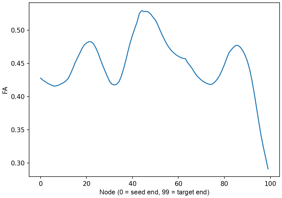
Note. FA peaks in deep white matter and declines toward the hippocampal end. VTA = ventral tegmental area.

Figure 2

NODDI Indices Along the Same Bundle

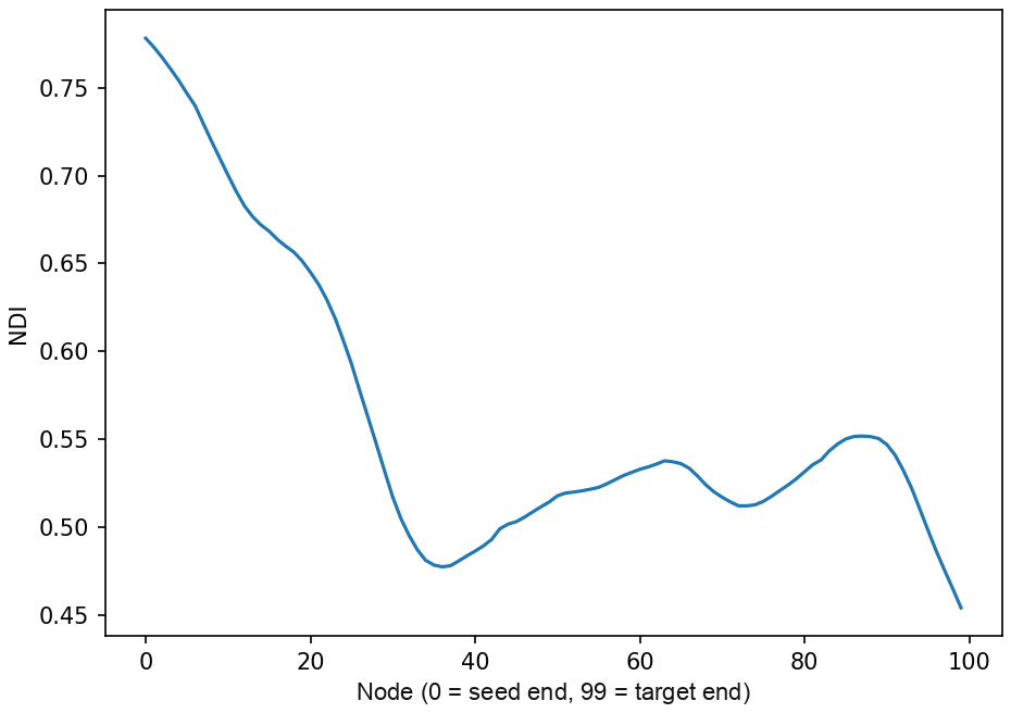
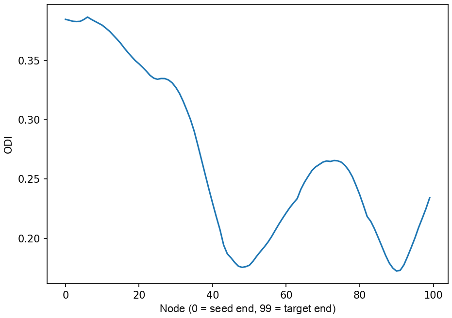
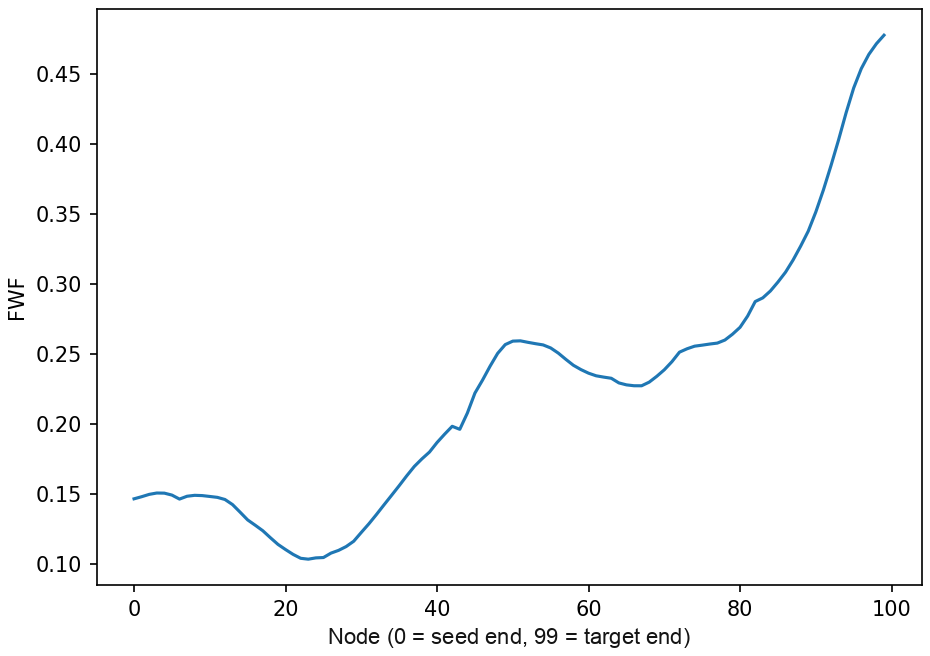
Note. NDI (top), ODI (middle) and FWF (bottom). NDI is high near the VTA and increases again toward the hippocampus; ODI is higher at both ends where fibres fan; FWF rises sharply at the hippocampal end adjacent to cerebrospinal fluid.

Figure 3

NDI Along the Anterior Tract for the Same Participant

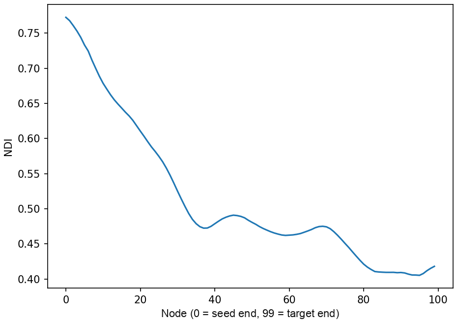
Note. The anterior tract shares the early trajectory and diverges late.

Verification

The row count of each CSV should equal the number of participants × 100.

When both hemispheres are processed, alignment should be confirmed before averaging. The across-participant correlation between node i on the left and node i on the right is strongly positive when the profiles are aligned and strongly negative when one side is reversed.